How to arrange Two excel sheets side by Side

Steps

• Click on View tab, Click on New Window
• Click on Arrange All, Select Vertical

Now to compare 2 Rows in 2 Excel Sheets

• Select the Rows in the Sheet which needs to be compared
• Click on Conditional Formatting Option
• =ISNA(MATCH(A2,Sheet2!A2,FALSE))

If you want the formatting to be applied only for one Column select that column and apply conditional formatting

Instead of

 =$A$2:$B$7

it should be

 =$A$2:$A$7

in Conditional Rules Formatting Manager

Download Excel

How to Filter cells based on Font Color, Cell Color

How to highlight rows which have different row value of one Column

The Steps are as Below
Below is the way to highlight the rows based on a change in value in the single column.The Column considered is SNo

Steps

• Select the whole DataSet LookUpArray on which the conditional formatting to be applied
• Click on Conditional Formatting
• Click on new Rule
• Use a formula to determine which cells to format
• Note : The formula used is relative formula =ISNA(MATCH($D2,$A$2:$A$7,FALSE))
• Use the format option to apply the Conditional format on the cells
• The same could be seen in Conditional Formatting->Manage Rules for future rule edits

In the below image Rows 4 and 7 are highlighted because of mismatch in SNo and 5 is highlighted because of mismatch in fruit name

Checking for Identical rows in two tables with more than one column

 =ISNA(MATCH($D2,$A$2:$A$7,FALSE)&MATCH($E2,$B$2:$B$7,FALSE) )

Steps

• First we are checking if the rows in D2 is same as on in A2 to A7
• Second we are checking if the rows in E2 is same as on in B2 to B7

=MATCH(lookup_value, lookup_array, match_type)

lookup_value – Value you are interested in
lookup_array – Column you want to look for value
match_type – Whether it should be a exact match or approximate match

Match Function

 =MATCH(D2,A2:A7,FALSE)

Looks for D2 in the Lookup Array in A2 to A7

Match with Msg

  =IFERROR(MATCH(D2,A2:A7,FALSE),"Missing")

In case of Error IFERROR is used to make it display as Missing

Match with ISNA

  =ISNA(MATCH(D2,A2:A7,FALSE))

If #N/A then it would be displayed as True

Match with 2 Columns

  =MATCH(D2,A2:A7,FALSE)&MATCH(E2,B2:B7,FALSE)

In the above code, we are checking the two columns for uniqueness by using two match function
and using && Operator to display the value as 11 or #N/A

formula to give you a comparison:

=AND(A2:A11=B2:B11)

Enter the formula by pressing Ctrl+Shift+Enter. If done correctly it will appear as the following:

{=AND(A2:A11=B2:B11)}

For a case-sensitive comparison, the equals operator will not work. Instead, the EXACT() function should be used.

{=AND(EXACT(A2:A11,B2:B11))}

VLOOKUP lets you search for specific information in your spreadsheet

Adding the arguments

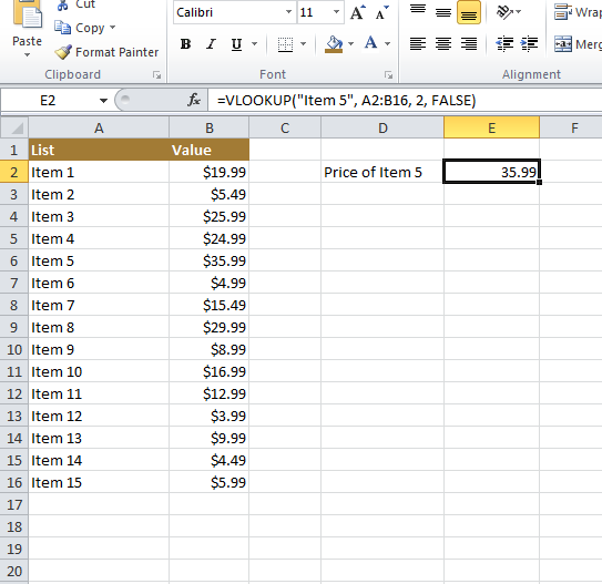
Now, we’ll add our arguments. The arguments will tell VLOOKUP what to search for and where to search.

The first argument is the name of the item you’re searching for, which in this case is Photo frame. Because the argument is text, we’ll need to put it in double quotes:

=VLOOKUP(“Item 5”

The second argument is the cell range that contains the data. In this example, our data is in A2:B16. As with any function, you’ll need to use a comma to separate each argument:

=VLOOKUP(“Item 5”, A2:B16

Note: It’s important to know that VLOOKUP will always search the first column in this range. In this example, it will search column A for “Item 5”. In some cases, you may need to move the columns around so the first column contains the correct data.

The third argument is the column index number. It’s simpler than it sounds: The first column in the range is 1, the second column is 2, etc. In this case, we are trying to find the price of the item, and the prices are contained in the second column. This means our third argument will be 2:

=VLOOKUP(“Item 5”, A2:B16, 2

The fourth argument tells VLOOKUP whether to look for approximate matches, and it can be either TRUE or FALSE. If it is TRUE, it will look for approximate matches. Generally, this is only useful if the first column has numerical values that have been sorted. Because we’re only looking for exact matches, the fourth argument should be FALSE. This is our last argument, so go ahead and close the parentheses:

=VLOOKUP(“Item 5”, A2:B16, 2, FALSE)

Finding Value of Particular Data

 =VLOOKUP("Item 5", A2:B16, 2, FALSE)

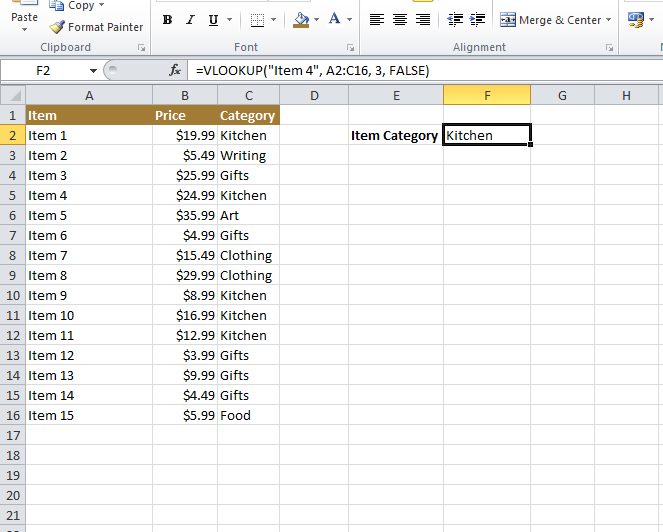
Finding Category in Two Columns

  =VLOOKUP("Item 4", A2:C16, 3, FALSE)

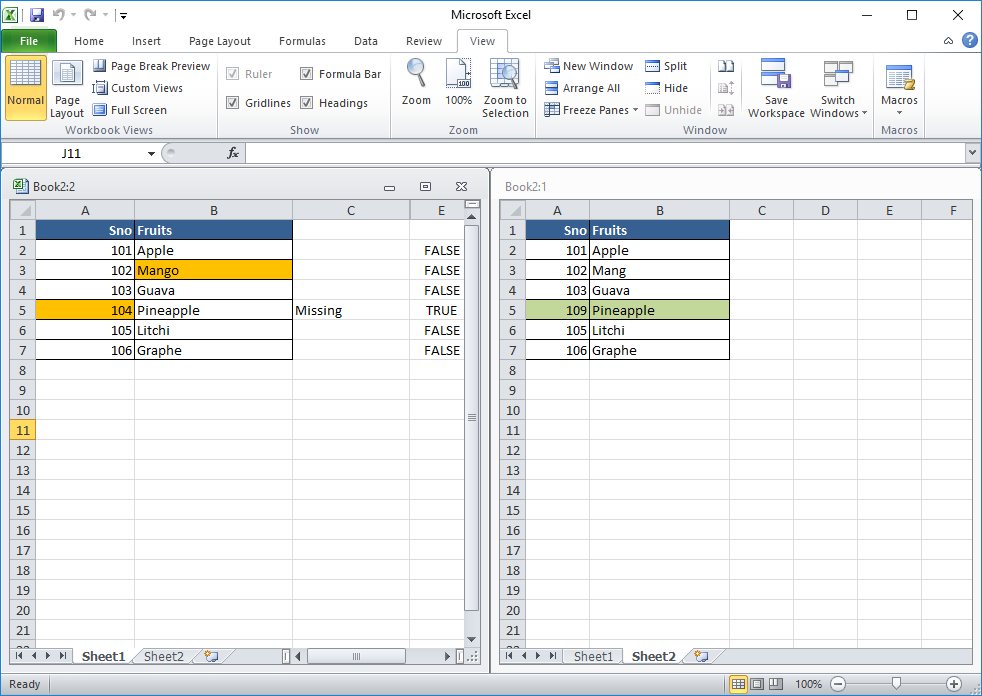
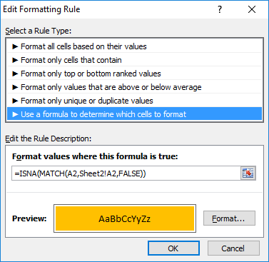
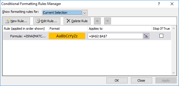
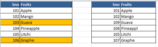
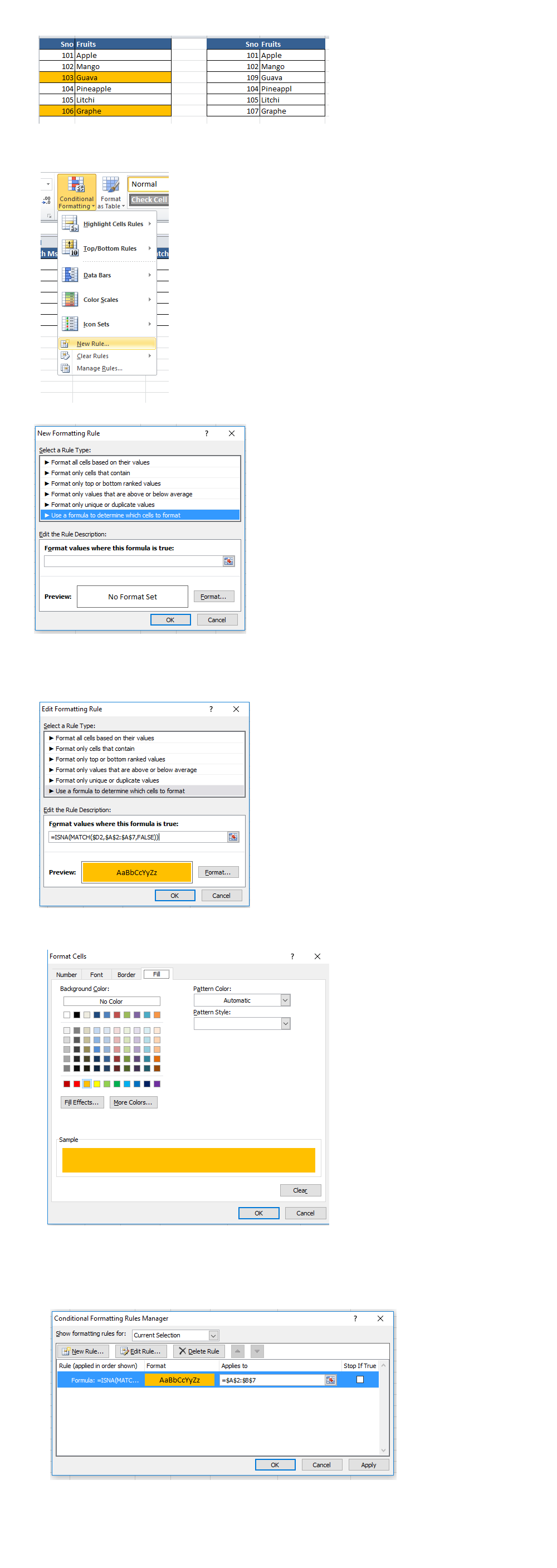
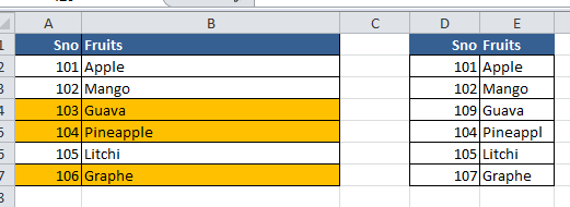
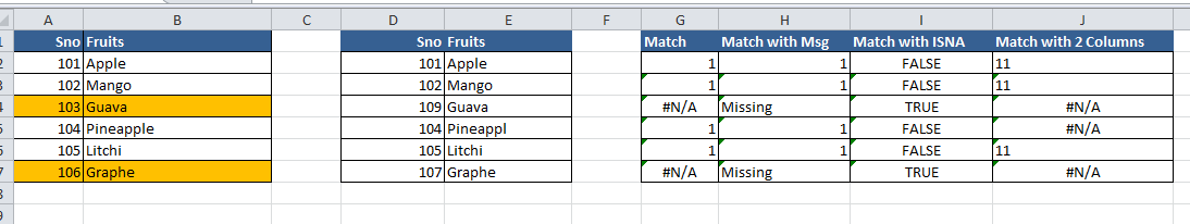
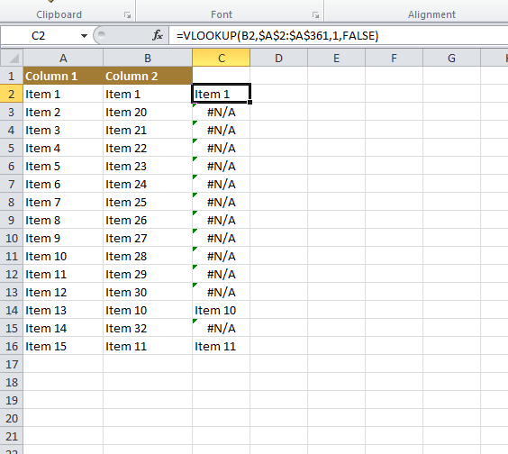
Finding Matching Data in Two Columns

   =VLOOKUP(B2,$A$2:$A$361,1,FALSE)

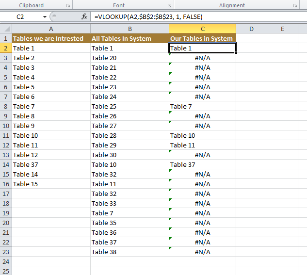
Filter Tables in System
The Super set column in which the sub set is searched should be added as a second parameter. In our case its B

   =VLOOKUP(A2,$B$2:$B$23, 1, FALSE)

There may be times where the excel date is displayed as number like one below. In such case the date can be converted to string as follows

Two things

1. The J column is aligned to Left which tells there is some custom format done over the cells
2. On selecting the cell and when you check the drop down at top it shows Custom

The Column K represents the actual value of Cells in J by making it to text format. Now to convert the Column J to Text use this simple excel formula

 =TEXT(A1,"DD/MM/YYYY hh:mm:ss")

 =CONCATENATE(B2,".",C2,".",D2)

--Update Script
  =CONCATENATE("UPDATE Location SET Location_Description = '", D2, "'  WHERE  LOCATION_CODE ='", B2,"' AND LOCATION_NAME ='", C2, "'")

 UPDATE Location 
   SET Location_Description = 'Thats where I Live'
 WHERE LOCATION_CODE = '600018'
   AND LOCATION_NAME = 'Teynampet'